
(Difference between revisions)
| Revision as of 15:36, 14 September 2006 Peter (Talk | contribs) (→An example) ← Previous diff |
Revision as of 15:36, 14 September 2006 Peter (Talk | contribs) (→An example) Next diff → |
||
| Line 22: | Line 22: | ||
| |width="300"|Select the variables you want to work with. For this example, select the variables TemJul, RnJul and RdJul. Clicking on the Ok button will start the calculations.||[[Image:grap86.jpg|grap86.jpg]] | |width="300"|Select the variables you want to work with. For this example, select the variables TemJul, RnJul and RdJul. Clicking on the Ok button will start the calculations.||[[Image:grap86.jpg|grap86.jpg]] | ||
| |---- | |---- | ||
| - | |width="300"|The output from the analysis is presented in two ways: as an output file, containing the values of the principal components themselves.||||[[Image:graph87.jpg|400px|]] | + | |width="300"|The output from the analysis is presented in two ways: as an output file, containing the values of the principal components themselves.||[[Image:graph87.jpg|400px|]] |
| |---- | |---- | ||
| - | |width="300"|Select the variables you want to work with. For this example, select the variables TemJul, RnJul and RdJul. Clicking on the Ok button will start the calculations.|| | + | |width="300"|Select the variables you want to work with. For this example, select the variables TemJul, RnJul and RdJul. Clicking on the Ok button will start the calculations. |
| ||[[Image:graph88.jpg|400px|]] | ||[[Image:graph88.jpg|400px|]] | ||
| |} | |} | ||
Revision as of 15:36, 14 September 2006
Calculating special crop indicators
Investigate parameters influencing Yield with Principal Components Analysis (PCA)
Principal components analysis is a powerful tool used to examine the structure of an input matrix containing the variables used in regression model building. As we are not certain whether the variables are independent of one another or whether they are important in explaining the variance in our yield, we can use principal components analysis to indicate variables with similar behaviours by redistributing the variance of the matrix among a new set of uncorrelated axes (the principal components). This analysis permits the replacement of the initial, generally correlated, variables by non-correlated ones. In addition, the analysis of the components often permits the reduction of a certain number of variables; one can, in effect, often cancel the third or sometimes even the second principal component of the three. The analysis also provides a complementary interpretation of the initial variables.
The correlations between the components and the original variables give some indications as to which variables are important, i.e., which variables are worth retaining in the multiple regression leading to the yield function.
An example
To illustrate how principal component analysis can be used, examine the input file SP-MET.DAT. The file contains annual yield from 1920 to 1930 and three climatological variables; the mean temperature, precipitation and radiation measured during the month of July. We imagine that the yield is a function of these three parameters but we suspect that the three variables are not entirely independent of one another. 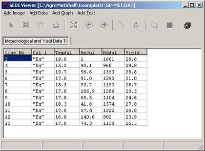
Activate the Tools - Principle Component Analysis function. A settings window appears. 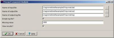
Select the variables you want to work with. For this example, select the variables TemJul, RnJul and RdJul. Clicking on the Ok button will start the calculations. 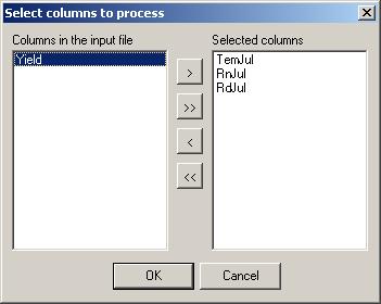
The output from the analysis is presented in two ways: as an output file, containing the values of the principal components themselves. 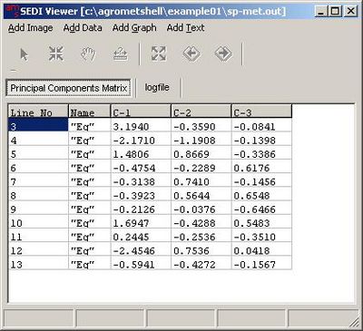
Select the variables you want to work with. For this example, select the variables TemJul, RnJul and RdJul. Clicking on the Ok button will start the calculations. 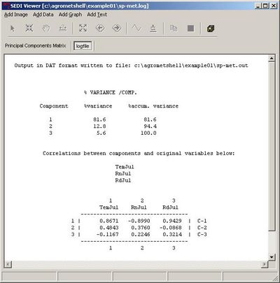
Calculating the Length of the Growing Period (LGP)
The length of the growing period (LGP), as defined by the Agro-Ecological Zones project carried out at FAO during the last two decades [refs], is the period (in days) during a year when precipitation exceeds half the potential evapotranspiration, plus a period required to evapotranspire an assumed 100 mm of water from excess precipitation stored in the soil profile.
The LGP is a useful concept for calculating agricultural potential, and can be used as a criterion for classifying areas and in roughly determining crop cycle lengths. The calculation of the growing period is based on a simple water balance model, comparing precipitation with PET, using monthly values. A "normal" growing period has the following characteristics:
- A Beginning. The beginning coincides with the start of the normal rainy season and is taken as the date when precipitation equals half PET, denoted as a in fig.5.4a. A value of 1/2 PET has been chosed because the water requirements of germinating crops are much below the full rate of PET, reflected clearly in the magnitude of the crop coefficients, and false starts to the rainy season are eliminated.
- A Humid Period. This is the period during which precipitation exceeds PET. The beginning and ending dates are the two points where the precipitation and PET curves cross. During this period, crops are able to meet their full water requirements and the soil moisture deficit is replenished. The ending date of the humid period coincides with the end of the rainy season and crops mature largely from water stored in the soil.
- An End to the Growing Period. This occurs at the point where the precipitation curve crosses the 1/2 PET curve (labeled as d in fig. 5.4a) and takes into consideration that most crops continue to grow beyond the end of the rainy season. The soil water-holding capacity (defined as....) is assumed to be 100 mm and the time taken to deplete the remaining soil reserves at the end of the season is added on to the LGP.
In addition to a normal period, three other types of growing periods can be defined:
- Intermediate Growing Period. Throughout the year, the average monthly precipitation does not exceed the full rate of the average monthly PET, but it does exceed half the PET. The beginning and the end of such an intermediate growing period are defined as the points where the precipitation curve crosses the 0.5 PET curve and there is no humid period.
- All Year Round Humid Growing Period. The average monthly pptn, for every month of the year, exceeds the full rate of the average monthly PET. Thus, there is no true start to the growing period or to the humid period. Areas with all year round humid growing periods have been included and inventoried as areas with a normal growing period of 365 days.
- All Year Round Dry Period. The average monthly precipitation for every month of the year is lower than half the average monthly PET. Areas with all year round dry periods have been inventoried separately as areas with a growing period of 0 days.
An example
Examine the sample data file, AL-LGP.DAT. The file contains station names in Africa, geographical coordinates between 2 North and 2 South, and 12 monthly values of rainfall and PET for each station. Notice that the input file requires the rainfall and PET to appear on the same line. 
Activate the Tools - Length of growing period function. A settings window appears and among other settings, you will be prompted to accept or change the default value of 1/2 PET to define the beginning and the end of the growing season as given in the original AEZ definition. For this example, accept the value and click on the Compute button to perform the calculation. 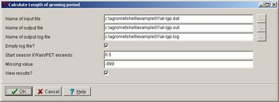
A new record of data (36 dekadal values for a year) can be entered after pressing the + sign in the toolbar at the top of the screen. In the next window, the station name can be entered. 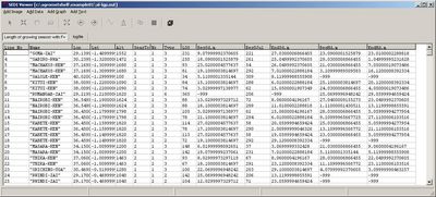
The first line of the file lists the limit you choose for determining the beginning and end of the growing season, i.e., 1/2 PET. This is followed by columns with the station name, latitude, longitude, altitude and several growing season characteristics. The next table describes the parameters in the output file and the range of possible answers:
Column Heading Meaning of the column variable Range of Answers Seastot Seasonal total rainfall (mm) N.A. Nr Number of seasons 1 - single; > 1 - multiple Type Type of season 1 - dry; 2 - intermediate; 3 - normal; 6 - normal with no dry period LGS Length of the Growing Season (days) 0 to 365 BegSd.m Beginning of the season (day.month) BegSJul Beginning of the season(Julian days) 0 to 365 EndSd.m End of the season (day.month) BegHd.m Beginning of the humid period (day.month) -999 if no humid period EndHd.m End of the humid period (day.month) -999 if no humid period
Note that for a station with a year round dry period, indicated as 1 under the column "Type", the LGS will be listed as having 365 days instead of 0 days.


