[edit]7.1. Calibrate crop yields against water balance outputs and other variables.
Peter Hoefsloot
In the context of agrometeorological crop yield forecasting, the yield function is a statistically derived function relating the water balance parameters (which constitute the outputs of the water balance model) and possibly other factors (like farm inputs, trend or NDVI) with station yield. Once this function has been established, it can be used for early crop yield forecasting for a number of seasons. Recalculation of this formula seems appropriate at least every 5 years to cater for changing climatological circumstances.Although many different equations are possible, the most widely used one is the outcome of a multiple linear regression procedure:
Y = a + b1X1 + b2X2 + b3X3where b1 to b3 are the corresponding X coefficients.
In this chapter an example for Malawi is used. In two steps the fomula will be calculated.
- Step 1. Determination of the water balance parameters which are good predictors for yield.
- Step 2. Performing the multiple linear regression.
The input data file for Malawi contains multiple lines for stations and years. The file is in FAO format and can be read by Excel as CSV file. In every line, besides yield, all possibly relevant water balance output parameters are stored. The file can be downloaded here 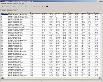
[edit]Step1. Finding the relevant parameters with a Principle Component Analysis (PCA)
Activate the Tools - Principle Component Analysis function. The settings window appears. 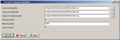
All parameters are selected to be included in the PCA analysis. 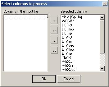
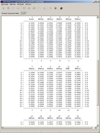
In this case, the output log file gives the most valuable results. Note that the first, second and third component explain over 50% of the variance. Therefore we will base the equation on these 3 components. 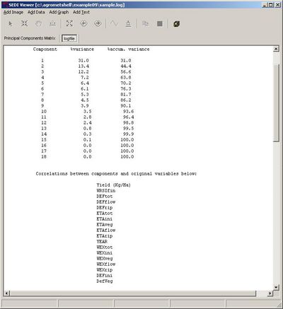
Within these components, the parameters with correlation above 0.70 or below -0.70 will be selected for use in the yield formula. This constitutes the following list:
- WRSIfin (final index)
- DEFtot (total deficit)
- DEFflow (total deficit during flowering)
- DEFrip (total deficit during ripening)
- ETAveg (ETA during vegetative stage)
- ETArip (ETA during ripening)
- WEXTot (Total Water Excess)
- WEXveg (Water excess during vegetative stage)
At the end of this first step, 8 parameters have been identified that will be part of the regression equation established in step 2.
[edit]Step 2. Performing the Linear Regression Analysis
The multiple regression is done in Excel. First the columns that are no longer needed are deleted. To prevent data loss the file is saved under the name sample1.xls. 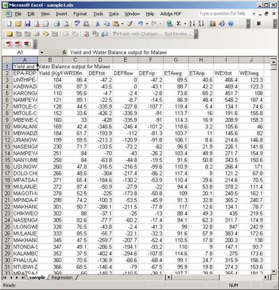
A second worksheet is created to hold the regression parameters. An array formula is entered : =LINEST(sample!B3:B1367,sample!C3:J1367, TRUE, TRUE)Now Excel calculates the regression parameters.
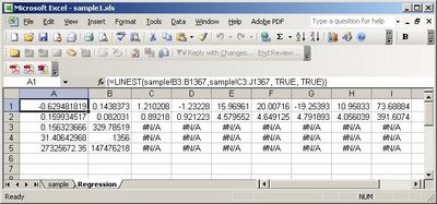
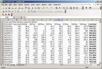
The parameters now lead to the following regression formula: yield = WRSIfin*10.95832936 + DEFtot*-19.25393401 + DEFflow*20.00715655 + DEFrip*15.96960614 + ETAveg*-1.232280314 + ETArip*1.210208146 + WEXtot*0.14383726 + WEXveg*-0.629481819 + 73.68884436The predected yield for the first data row (third line) is:
=Regression!A$1*J3+Regression!B$1*I3+Regression!C$1*H3+Regression!D$1*G3+Regression!E$1*F3+Regression!F$1*E3+Regression!G$1*D3+Regression!H$1*C3+Regression!I$1
A graph is created in which measured and predicted yield are combined. This gives an idea of the accurracy of the regression formula calculated. In this case correlation is rather poor. The sample workbook (sample1.xls) can de downloaded here 

| CM Box User Guide | Main Page | About | Special pages | Log in |
Printable version | Disclaimer | Privacy policy |


