[edit]5.2. Filling gaps in agricultural statistics.
René Gommes, Linda See, Peter Hoefsloot
[edit]Examples of “missing” statistical data
National agricultural statistics data are easily available, as they are published by the countries as statistical yearbooks and systematically assembled by FAO into the annual Production Yearbooks (FAOSTAT). Sub-national data, on the other hand, are usually difficult to retrieve, and subject to a number of complications when they have to be consolidated into a homogeneous and consistent set at the continental level.
It occurs rather often that the data are scarce or unavailable altogether. Possible causes:
- no sampling is carried out at the national level. Sometimes subjective estimates are produced, but they are of uncertain quality;
- data are collected at the national level, but never documented or actually published in national statistical yearbooks. However, some of those data are available nationally from the concerned services;
- different data are collected for different geographic units (for instance, not all Administrative Units collect data for all crops, or sometimes the different Administrative Units apply for agriculture and, say population;
- data are aggregated (by areas or by crops) in a way which is not compatible with the reporting of other countries. A typical example would be “millet” which can be bulrush millet or finger millet, or both together, although the crops are rather different from an auto-ecological point of view. The worst example being “millet and sorghum” reported as either “millet” or “sorghum”;
- the Administrative Unit units were modified during the reference period. This creates a minor difficulty when Administrative Unit are aggregated, but when they are split, it is not always possible to redistribute the statistics between the new Administrative Unit;
- crops are not reported on separately, for instance white potatoes can sometimes be lumped with vegetables and appear nowhere in the statistics.
- etc..
Fortunately, a number of techniques exist to estimate missing data.
[edit]Examples of strategies for filling gaps in maps
A number of methods can be applied to fill gaps. It depends on the agricultural parameter at hand, which methods are applied. Usually a sequence of methods is necessary. Some examples of a possible sequence of methods are given below.
Production
- Disaggregation of national production
- Spatialization of per capita production x Administrative Unit population
- Administrative Unit yield x Administrative Unit cropped area
Yield
- Regression against environmental variable
- Inverse-distance spatialization
- SEDI interpolation
Cropped Area
- Disaggregation of national cropped area
- Spatialization of area per capita x Administrative Unit population
- Spatialization of relative area x Administrative Unit total area
Considering, for instance, that Administrative Unit yield can be derived using three methods and that cropped area can also be derived with different approaches, the number of “final” values is thus rather high. Also consider that sums can be estimated as sums (“coarse grains”) and as the individual components (i.e. maize, barley, millet, sorghum etc.), which in turn add another set of possible values. Whenever the estimates are reasonably close, they can be averages without much afterthought... but when they differ by an order of magnitude, subjective choices have to be made.
Therefore, the results are user-dependent and they result from a set of common-sense rules rather than from a method as such. It is assumed that the methods used as well as the harmonization with FAOSTAT ensures that the final product is consistent.
[edit]Description of Methods
[edit]Disaggregation of quantities
Disaggregation consists in re-distributing the total national production or areas in proportion to some other known variable, for instance population. This can be applied only if the country is relatively homogeneous from an agroecological point of view.
[edit]Inverse distance weighting
Geostatistical interpolation of missing data consists in the estimation of missing values at one point in space based on the known values of neighboring entities. The inverse-distance weighting is one of the most straightforward methods; it takes into account the distance between the “known” and “unknown” points and their relative importance in the estimation. For instance, close-by Administrative Units of the same country are assigned a higher weight than the Administrative Unit’s of neighboring countries distance. The reason for this is that it is considered that production and feeding behavior are more homogeneous within the country.
For the geo-statistical interpolation, it can generally be considered that reported crop yield corresponds to the centre of gravity of the Administrative Unit. The AgrometShell function Tools-Interpolate to replace missing data can be used to perfome this type of operation.
[edit]External variables useable for spatial interpolation
Is is possible to use pixel-based information that is generally available from non-national sources, like satellite imagery, or topographic information from digital terrain models, etc., to assist with the estimation of the missing statistical information by administrative unit (Administrative Unit).
As indicated, the spatial interpolation can either be purely geo-statistical, or take advantage of the additional knowledge obtained from external variables. In the first category falls the method known as inverse distance weighting (described above). In the second, the method was Satellite Enhanced Data Interpolation (SEDI).
In semi-arid areas, good correlations can be found between environmental conditions and yield (K/H). Once average Administrative Unit values of NDVI, elevation, etc. are available for surrounding areas, yields can be regressed against the external environmental variables . The method is not applicable if cultivars vary in the same agroclimatic area. Generally this information is not included in the statistics, and the database was thus considered cultivar- independent.
For crop forecasting, an important external variable of interest is NDVI (Normalized Difference vegetation Index), regularly available every 10 days since 1981. It represents one of the most popular remotely sensed indicators for monitoring the response of vegetation to weather condition in several parts of Africa.
NDVI is an indicator of the density of living green mass; in theory, it varies from -1 to +1, but in practice only values between 0 to 0.7 are found on land areas.
As an example the figure below illustrates a typical relation between yield and NDVI, showing, among others, NDVI values starting at about 0.07 and yields leveling off from values above 0.2. Note that the values indicated correspond to the spatial average over a whole Administrative Unit, where no crops are actually grown below about 0.12. This explains why relatively high yields can be found at low NDVI when some crops are irrigated or grown in the wettest parts of the Administrative Unit only.
Coarse grain yield and NDVI in Burkina Faso and the countries surrounding Burkina Faso. The figure was restricted to yields below 1200 Kg/Ha. 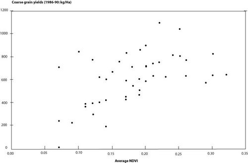 [edit]
Satellite Enhanced Data Interpolation, or SEDI
SEDI takes advantage of the correlation between and environmental variable, for instance the above mentioned NDVI/biomass and agricultural yields. One of the ways to approach this is co-kriging, a variant of kriging using one or more ausiliary variable and exploiting both the spatial features of the variable to be interpolated and the correlations between the variable and the ausiliary variables.
The SEDI interpolation method originated in a Harare based FAO Regional Remote Sensing Project. It was originally developed to interpolate rainfall data collected at station level using the additional information provided by METEOSAT cold cloud duration images. The methods proved powerful and versatile, and it is now regularly used by FAO to spatially interpolate other parameters as well (e.g. potential evapotranspiration, crop yields, actual crop evapotranspiration estimates etc.
SEDI is a simple and straightforward method for 'assisted' interpolation. The method can be applied to any parameter of which the values are available for a number of geographical locations, as long as a 'background' field is available that has a negative or positive relation to the parameter that needs to be interpolated.
Three requirements are a prerequisite for the successful application of the SEDI method:
- The availability of the parameter to interpolate as point data at different geographical locations (e.g. rainfall, potential evapotranspiration, crop yields).
- The availability of a background parameter in the form of a regularly spaced grid (or field) for the same geographical area (e.g. the above-mentioned NDVI variables , altitude).
- A relation between the two parameters (negative or positive; Yield/NDVI is positive, temperature/altitude would be negative). A Spearman rank correlation test can reveal whether a relation exists, and how strong this relation is.
The SEDI method yields the parameter mentioned under point 1 as a field (i.e. an image covering the whole area under consideration. The average of the field value over the Administrative Unit provides the estimation of the spatialized statistic.
A detailed description of the SEDI method can be found here

| CM Box User Guide | Main Page | About | Special pages | Log in |
Printable version | Disclaimer | Privacy policy |
